EVE results analysis
Lars Grønvold
19/06/2020
OGtbl <- read_tsv("input-data/from_ortho_pipeline/OGtbl.tsv",col_types = cols())

# load the expression data
combExprMat <- readRDS("data/BSNormalize/combExprMat.RDS")

# raw expression data
exprsMat <- readRDS("input-data/RNAseq/exprsMat.RDS")

# load EVE results
EVEresTbl <- readRDS("data/runEVE/EVEresTbl.RDS")
The orthogroups
Orthogroups (OGs) are based on the gene trees from the ohnolog pipeline. The trees are split into teleost clades (internal node “N3” in the species tree) and filtered based on the phylogeny and gene copy-numbers:
- No out-group paralogs, i.e. Max 1 gene per out-group species (Drer, Olat, Eluc) per N3 clade
- No salmonid paralogs, i.e. Max 1 gene per in-group/salmonid species (Ssal, Salp, Omyk, Okis) in each of the salmonid clade (N9)
- Either 1 (singleton) or 2 (duplicate) salmonid clades (N9)
- One salmonid ortholog must be expressed (one or more mapped RNA-seq reads).
- The Eluc ortholog and either Drer or Olat must be expressed.
EVE results
Theta shifts
Overview statistics of the EVE results. Shows the proportion of significant shifts up and down.
# When combining 1:1 and 1:2 into one plot the "both" category only occurs for duplicates and
# will either show  up in all facets or the bars will have different widths.
# Here is a workaround for dealing with the widths..

# scale facets based on the number of categories in each
drawBalancedBarsFlipped <- function(p){
  # convert ggplot object to grob object
  gp <- ggplotGrob(p)

  # # optional: take a look at the grob object's layout
  # gtable::gtable_show_layout(gp)

  # get gtable rows corresponding to the facets
  facet.rows <- gp$layout$b[grepl("panel", gp$layout$name)]

  # get the number of unique x-axis values per facet (1 & 3, in this case)
  x.var <- sapply(ggplot_build(p)$layout$panel_scales_x,
                  function(l) length(l$range$range))

  # change the relative widths of the facet columns based on
  # how many unique x-axis values are in each facet
  gp$heights[facet.rows] <- gp$heights[facet.rows] * x.var

  # plot result
  grid::grid.draw(gp)
}
Ntbl <-
EVEresTbl %>%
mutate( isComplete = ifelse(N3partial,"partial","full") ) %>%
select(N3, isComplete,dup_type) %>% distinct() %>% count(isComplete,dup_type) %>%
mutate(N=paste("N =",n))
EVEresTbl %>%
mutate( sigDir = ifelse(dup_type=="single",sigDir,dupSigDir)) %>%
mutate( isComplete = ifelse(ifelse(dup_type=="single",N9partial,N3partial),"partial","full") ) %>%
select(N3,sigDir,dup_type,isComplete) %>%
distinct() %>%
add_count(dup_type,isComplete) %>%
# mutate( category = paste0(dup_type,isComplete," (n=",n,")")) %>%
filter( sigDir != "" ) %>%
group_by( sigDir, dup_type,isComplete) %>%
summarise(nSig = n(), N=n[1], propSig=n()/n[1]) %>%
mutate( updownClass = sub(x = sigDir,"(up|down|both).*","\\1")) %>%
group_by(updownClass,dup_type, isComplete) %>%
arrange(desc(sigDir)) %>%
mutate(totSig=cumsum(propSig)) %>%
rename( Direction=sigDir) %>%
ggplot( aes(x=updownClass, y=propSig) ) +
geom_col(aes(fill=Direction)) +
facet_grid( dup_type ~ isComplete,scales = "free" ) +
scale_fill_manual(values = c(both="#993094",down="#298ABD",downdown="#1B4F8B",
up="#F62D31",upup="#8B1B1A")) +
geom_text(aes(label=nSig,y=totSig),hjust=-0.1 ) +
coord_flip(ylim = c(0,0.4)) +
geom_text(data=Ntbl,mapping = aes(label=N),y=0.4,x=1, hjust=1) +
ylab("Proportion of OGs with expression shift") +
theme_classic() +
theme(axis.title.y = element_blank()) -> p
drawBalancedBarsFlipped(p)
Bias towards partially retained
Compare results for duplicate clades where one clade is complete and the other has lost one or more orthologs (i.e. partial). The ohnolog clade with loss is more likely to be downregulated
EVEresTbl %>%
  filter(dup_type=="duplicate") %>%
  group_by(N3) %>%
  # find ortholog groups where one of the clades are partial
  filter( sum(N9partial)==1) %>%
  ungroup() %>%
  select( N3, N9partial, sigDir )  %>%
  mutate( isComplete = ifelse(N9partial,"partial","full") ) %>%
  add_count(isComplete) %>%
  group_by(isComplete, sigDir) %>%
  summarise(nSig = n(), N=n[1], propSig=n()/n[1]) %>%
  filter( sigDir!="") %>%
  ggplot( aes(x=sigDir, y=propSig,fill=sigDir) ) +
  geom_col() +
  facet_grid( isComplete ~ ., scales = "free_x" ) +
  scale_fill_manual(values = c(down="#298ABD",downdown="#1B4F8B",
                              up="#F62D31",upup="#8B1B1A")) +
  geom_text(aes(label=nSig),hjust=-0.1 ) +
  coord_flip(ylim = c(0,0.4)) +
  annotate("text",x=2,y=0.4,label="N = 1775",hjust=1) +
  theme_classic() +
  theme(legend.position = "none")
Both clades partial
EVEresTbl %>%
  filter(dup_type=="duplicate") %>%
  group_by(N3) %>%
  # find ortholog groups where both of the clades are partial
  filter( all(N9partial)) %>%
  ungroup() %>%
  select( N3, dupSigDir )  %>%
  distinct() %>%
  mutate(n=n()) %>%
  filter( dupSigDir!="") %>%
  group_by(dupSigDir) %>%
  summarise(nSig = n(), N=n[1], propSig=n()/n[1]) %>%
  mutate( updownClass = sub(x = dupSigDir,"(up|down|both).*","\\1")) %>%
  group_by(updownClass) %>%
  arrange(desc(dupSigDir)) %>%
  mutate(totSig=cumsum(propSig)) %>%
  rename(Direction=dupSigDir) %>%
  ggplot( aes(x=updownClass, y=propSig) ) +
  geom_col(aes(fill=Direction)) +
  scale_fill_manual(values = c(both="#993094",down="#298ABD",downdown="#1B4F8B",
                              up="#F62D31",upup="#8B1B1A")) +
  geom_text(aes(label=nSig,y=totSig),hjust=-0.1 ) +
  coord_flip(ylim = c(0,0.4)) +
  annotate("text",x=1,y=0.4,label="N = 743",hjust=1) +
  ylab("Proportion of OGs with expression shift") +
  theme_classic() +
  theme(axis.title.y = element_blank())
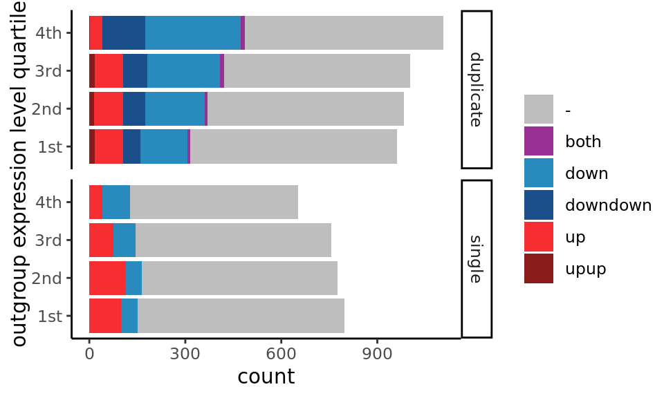
Expression level bias on expression shift detection
outgroup_cols <- colnames(combExprMat) %in% c("Drer","Olat","Eluc")

EVEresTbl %>%
  left_join(
    tibble(
      N9 = rownames(combExprMat),
      outgroup = rowMeans(combExprMat[ , outgroup_cols],na.rm = T)
    ), by="N9"
  ) %>%
  filter(N3partial==F) %>%
  select(N3,dupSigDir,dup_type,outgroup) %>%
  distinct() %>%
  mutate( quartile=cut(outgroup, breaks = quantile(outgroup),
                       include.lowest = T,labels = c("1st","2nd","3rd","4th"))) %>%
  add_count(dup_type) %>%
  mutate( dupSigDir = ifelse(dupSigDir=="","-",dupSigDir) ) %>%
  ggplot( aes(x=quartile,fill=dupSigDir)) +
  facet_grid( dup_type ~ .) +
  geom_bar() +
  scale_fill_manual(values = c(both="#993094",down="#298ABD",downdown="#1B4F8B",
                              up="#F62D31",upup="#8B1B1A",`-`="grey"), name="")+
  coord_flip() +
  theme_classic() +
  xlab("outgroup expression level quartile")